


Welcome back to my portfolio blog. After previously working on a simple POS system using Python and building business insights dashboards using Power BI, in this project I continue exploring the data analysis workflow using Python, especially for data cleaning and exploratory data analysis (EDA).
In this article, I am working with the Club Member Dataset, where I focus on preparing raw data, handling missing values, identifying inconsistencies, and visualizing patterns using several common visualization techniques such as boxplots, lineplots, histograms, and correlation analysis. Through this project, I want to demonstrate how Python libraries such as Pandas and Seaborn can help transform raw datasets into meaningful visual insights.
Project Overview
Dataset Overview
The dataset I used consists of a single CSV file, club_member_info.csv, which contains various details about club members. It includes personal, contact, and membership-related information. The original dataset contains the following columns:
- full_name (text): Member’s complete name stored in a single column
- age (integer): Member’s age, although some entries contain extra digits
- marital_status (text): Member’s marital status
- email (text): Unique email address for each member
- phone (text): Contact phone number
- full_address (text): Combined address including street, city, and state
- job_title (text): Member’s occupation
- membership_date (date): Date the member joined the club (all entries are within the 2000s)
Tech Stack
- Python
- Pandas
- NumPy
- Matplotlib
- Seaborn
- Jupyter Notebook
Short Summary
After completing the data cleaning process, I generated a brief statistical summary to better understand the dataset:
- Age: I find that the average age is approximately 41.7, with a minimum of 18 and a maximum of 68 after correcting invalid entries.
- Marital Status: I find that the average number of records with the “Married” status is 877, while the lowest number is for “Separated,” with 167 records
- Membership Timeline: All membership dates fall within the 2000s, indicating that the dataset represents relatively recent members.
- Data Completeness: I standardize missing values by converting empty fields into NULL to ensure consistency.
- Uniqueness: I remove duplicate records by using the email column, ensuring that each member is uniquely represented.
Solution Approach: Data Cleaning
Part 1: Data Understanding
In the first stage of this project, I started by importing the main Python libraries required for data analysis (NumPy and Pandas). To ensure the original dataset remained unchanged during the cleaning process, I created a backup copy of the dataset using the .copy() method. This is important because it allows me to experiment safely without modifying the raw data directly.
Next, I performed an initial data understanding process to explore the overall structure and quality of the dataset. In this stage, I examined:
- The first five rows of the dataset using .head()
- General dataset information using .info()
- The number of non-null values in each column using .count()
- Statistical summaries for numerical columns using .describe()
- Category distribution for the martial_status column using .value_counts()
I added a custom id column to create a unique identifier for each record and then set it as the DataFrame index.
#1. section ini berisi import dan data mentah
import numpy as np
import pandas as pd

raw_data = pd.read_csv("D:/Documents/Projectku/Data Analyst/Python/Projek Club Member/python-club_member_info.csv")
df = pd.DataFrame(raw_data)

#membuat backup data
club = df.copy()

#2.  section ini berisi Data Understanding
print("1. Ambil 5 baris data sebagai ringkasan\n\n", club.head(), "\n\n")
print("2. Struktur data secara umum", club.info(), "\n\n")
print("3. Struktur data per kolom\n\n", club.count(), "\n\n")
print("4. Struktur data kolom Age (Numerikal)\n\n", club.describe(), "\n\n")
print("5. Struktur data untuk kolom martial status\n\n", club["martial_status"].value_counts(dropna=False))

#3. penambahan kolom ID
club["id"] = range(1, len(club)+1)
club = club.set_index("id")
print(club.tail())Before proceeding with the cleaning stage, I also categorized the columns based on their level of importance in the dataset.
- Mandatory Fields
These columns are considered essential and must contain valid data. Rows with missing values in these fields may need to be removed because they are critical for identification and analysis purposes.
- email — used as a unique identifier
- membership_date
- Optional Fields
These columns are not strictly required for the analysis process. Missing values in these fields can still be tolerated, although further confirmation from the client or data provider may be necessary if the missing data becomes significant.
- full_name
- age
- martial_status
- phone
- full_address
- job_title
Part 2: Data Error Identification
In this stage, I focused on identifying potential errors and inconsistencies in each column before performing the actual cleaning process. Generally, I checked every column for several common data quality issues, including:
- Missing values (NA)
- Unusual or invalid characters — except for the email column
- Empty string values (”)
In addition, I applied several specific validation techniques depending on the column type and business rules.
- Additional Validation Checks
- Range validation — specifically for the age and membership_date columns
- Invalid format validation — mainly for the membership_date column
- Categorical value validation — for the martial_status column
- Duplicate checking — specifically for the email column
- Membership date validation — checking dates that are greater than the current year or earlier than the year 2000
#4.1 full_name
fn_cek_na = club["full_name"].isna().sum()
fn_cek_strange = club["full_name"].str.contains(r"[^a-zA-Z' -]")
print(f"total baris NA: {fn_cek_na}")
print(f"total baris dengan karakter aneh (bukan huruf/strip/apostrof): {fn_cek_strange.sum()}")
print(club[fn_cek_strange])

#4.2 age
age_cek_na = club["age"].isna().sum()
age_cek_strange = club["age"].astype("str").str.match(r"^\d+$", na=False).sum()
age_cek_valid = club["age"] > 100
print(f"total baris NA: {age_cek_na}")
print(f"total baris dengan karakter aneh: {age_cek_strange}")
print(f"total baris dengan usia di atas 100 tahun: {age_cek_valid.sum()}")

#4.3 martial status
ms_cek_na = club["martial_status"].isna().sum()
ms_cek_catvalid = club["martial_status"].value_counts(dropna=False)
print(f"jumlah data NA: {ms_cek_na}")
print(f"\ndistribusi kategorikal:\n{ms_cek_catvalid}")
print("\nada kesalahan pengisian di mana divored harusnya divorced")

#4.4 email: melihat data duplikat
email_cek_na = club["email"].isna().sum()
email_cek_duplikat = club.duplicated(subset="email", keep=False).sum()
print(f"total baris NA: {email_cek_na} baris")
print(f"total baris duplikat: {email_cek_duplikat} baris")

#4.5 phone
phone_cek_na = club["phone"].isna().sum()
phone_cek_strange = club["phone"].str.contains(r"[^0-9+\-\s()]").sum()
phone_kar_lebih = (club["phone"].str.len() < 8) | (club["phone"].str.len() > 14)
print(f"total baris NA: {phone_cek_na} baris")
print(f"total baris karakter nomor hp aneh: {phone_cek_strange} baris")
print(f"total baris phone yang lebih invalid (8 digit < karakter > 14 digit): {phone_kar_lebih.sum()} baris")

#4.6 full_address
fa_cek_na = club["full_address"].isna().sum()
fa_cek_strange = club["full_address"].str.contains(r"[^a-zA-Z0-9\s.,+/#-]").sum()
print(f"total baris NA: {fa_cek_na} baris")
print(f"total baris dengan karakter aneh: {fa_cek_strange} baris")

#4.7 job_title
jt_cek_na = club["job_title"].isna().sum()
jt_cek_strange = club["full_address"].str.contains(r"[I|II|III|IV]").sum()
print(f"total baris NA: {jt_cek_na} baris")
print(f"total baris dengan karakter aneh: {jt_cek_strange} baris")

#4.8 membership_date -- terlebih dahulu ubah ke format tanggal
md_cek_nontanggal = club["membership_date"].astype("str").str.contains(r"[^0-9\-/]").sum()
club["membership_date"] = pd.to_datetime(club["membership_date"])

md_cek_na = club["membership_date"].isna().sum()
md_cek_invalid = club["membership_date"] > pd.Timestamp.today()
md_cek_lama = club["membership_date"].dt.year < 2000

print(f"Jumlah baris dengan data bukan tanggal: {md_cek_nontanggal}")
print(f"jumlah baris dengan tanggal aneh (lebih dari hari sekarang): {md_cek_invalid.sum()}")
print(f"jumlah baris dengan tanggal aneh (di bawah tahun 2000): {md_cek_lama.sum()}")
print(f"total baris NA: {md_cek_na} baris")
print(club[md_cek_lama])
print(club["membership_date"].dt.year.value_counts().sort_index())After performing the identification process, I found several issues across the dataset.
- full_name: The full_name column contained many invalid characters outside alphabetic characters, hyphens, apostrophes, and spaces. In total, I found 52 problematic records. In addition, the name formatting was inconsistent, including lowercase formatting, capitalization inconsistencies, and unnecessary leading spaces at the beginning of names.
- age: There were 3 rows with missing values in the age column. I also discovered 15 records with unrealistic ages above 100 years old. Most of these issues were caused by duplicated number inputs, such as 455 instead of 45.
- martial_status: The martial_status column contained 20 missing values and several category inconsistencies caused by typing errors. Additionally, I identified that the column name itself was incorrect and should have been written as marital_status.
- email: I found 19 duplicated email records. Since email functions as a unique identifier in this dataset, duplicate values needed special attention during the cleaning process.
- phone: The phone column contained 9 rows with missing values.
- full_address: For the full_address column, the main task was not error correction but data transformation. I separated the address information into three individual columns: street_address, city, and state.
- job_title: The job_title column contained 39 missing values and around 380 rows with unusual characters, especially Roman numerals such as I, II, III, and IV.
- membership_date: I discovered several invalid dates in the membership_date column. In total, there were 16 records with dates incorrectly stored in the 1900s, which did not match the expected membership timeline for this dataset.
Part 3: Data Cleaning
After identifying the errors and inconsistencies in the dataset, I continued with the actual data cleaning process.
- full_name
For the full_name column, I removed unusual characters that were not relevant for personal names. I also standardized the formatting by converting each word into proper title case (capitalizing the first letter of each word) and removing unnecessary leading or excessive spaces.
- age
In the age column, some invalid values were caused by repeated digit patterns such as 455 instead of 45. Since the errors followed a repetitive pattern, I used regular expressions (regex) to identify and replace the duplicated number patterns automatically.
- martial_status
I corrected category inconsistencies in the martial_status column by replacing incorrect values such as divored with the correct category, divorced.
Because the email column functions as a unique identifier, duplicated records needed to be removed.
- phone
No cleaning process was applied to the phone column. Based on the data validation rules defined earlier, this column was categorized as an optional field, meaning missing values were still acceptable within the scope of this project.
- full_address
The full_address column was transformed by splitting the address information into separate columns to improve readability and analysis flexibility. The address was divided into street_address, city, and state.
- job_title
For the job_title column, I removed Roman numeral characters such as I, II, III, and IV from the strings to make job title naming more standardized and consistent.
- membership_date
Several invalid dates were found in the membership_date column, especially records mistakenly stored in the 1900s. To fix this issue, I adjusted the incorrect years by adding 100 years to the affected records, converting them into dates within the 2010+ range that better matched the expected membership timeline.
#membuat copy data untuk langkah preventif
clubku = club.copy()

#5.1 duplicate handling
club = club.drop_duplicates(subset="email", keep="first")
data_duplikat = club.duplicated(subset="email", keep=False)
print(f"jumlah data duplikat sekarang: {data_duplikat.sum()}")

#full_name
fn_strange = club["full_name"].str.contains(r"[^a-zA-Z' -]")
club.loc[fn_strange, "full_name"] = club.loc[fn_strange, "full_name"].str.replace(r"[^a-zA-Z' -]","", regex=True)
club["full_name"] = club["full_name"].str.title()
club["full_name"] = club["full_name"].str.strip()

print(f"jumlah karakter aneh sekarang: {fn_strange.sum()}")
print(club["full_name"].sample(10))

#age
club["age"] = club["age"].astype("Int64") #ubah ke format integral bukan float
age_ganda = club["age"].astype(str).str.contains(r"\d{3}")
club.loc[age_ganda, "age"] = club.loc[age_ganda,"age"].astype(str).str[:2].astype(float)
print(age_ganda.sum())

#marital_status
club.rename(columns={"martial_status":"marital_status"}, inplace=True)
ms_divored = club["marital_status"].str.contains("divored", na=False)
club.loc[ms_divored, "marital_status"] = club.loc[ms_divored, "marital_status"].str.replace("divored", "divorced")
print(ms_divored.sum())

#full_address
club[["street_address", "city", "state"]] = club["full_address"].str.split(",", expand=True)
# Reorder kolom
club = club[["full_name", "age", "marital_status", "email", "phone", "full_address", "street_address", "city", "state", "job_title", "membership_date"]]
print(club.head())

#job_title
jt_strange = club["job_title"].str.contains(r"[I|II|III|IV]$", na=False)
club.loc[jt_strange, "job_title"] = club.loc[jt_strange, "job_title"].str.replace(r"\s*(I|II|III|IV)$","", regex=True)
print(f"jumlah karakter aneh sekarang: {jt_strange.sum()}")

#membership_date
md_lama = club["membership_date"].dt.year < 2000
club.loc[md_lama, "membership_date"] = club.loc[md_lama, "membership_date"] + pd.DateOffset(years=100)
print(club[md_lama])Solution Approach: Exploratory Data Analysis (EDA)
1. Univariate Analysis
In this section, I explored individual variables to understand their distributions, frequencies, and overall patterns. Analysis performed are Age distribution, Marital status distribution, City distribution, State distribution, and Job title distribution
#1. section ini berisi import dan data mentah
import numpy as np
import pandas as pd
import seaborn as sns
import matplotlib.pyplot as plt

dataku = pd.read_csv("D:/Documents/Projectku/Data Analyst/Python/Projek Club Member/clean-club_member_info.csv")

# Set tema grafik
sns.set_theme(style="whitegrid")
plt.figure(figsize=(10, 6))

#2. section ini berisi analisis Univariate
#Analisis Age
plt.figure(figsize=(10,8))

plt.subplot(2,1,1)
sns.histplot(data=dataku, x="age", bins=13)
plt.title("Distribusi Umur", fontsize=14, fontweight="bold", pad=20)
plt.xticks(range(20,70,10))

plt.subplot(2,1,2)
sns.boxplot(data=dataku, x="age", width=0.5)
plt.title("Outlier Pada Umur", fontsize=14, fontweight="bold", pad=20)

plt.tight_layout()

#marital_status (diurutkan dari terbanyak)
tb = dataku["marital_status"].value_counts().index
sns.countplot(data=dataku, x="marital_status", order=dataku["marital_status"].value_counts().index)
plt.title("distribusi status pernikahan", fontsize=14, fontweight="bold", pad=20)

#city
sns.countplot(data=dataku, x="city", order=dataku["city"].value_counts().head(10).index)

plt.xticks(rotation=45)
plt.title("distribusi 10 kota terbanyak", fontsize=14, fontweight="bold", pad=20)

#state
sns.countplot(data=dataku, x="state", order=dataku["state"].value_counts().head(10).index)

plt.xticks(rotation=45)
plt.title("distribusi 10 negara bagian terbanyak", fontsize=14, fontweight="bold", pad=20)

#job_title
plt.figure(figsize=(6,3))
sns.countplot(data=dataku, x="job_title", order=dataku["job_title"].value_counts().head(10).index)

plt.xticks(rotation=90)
plt.title("distribusi 10 pekerjaan terbanyak", fontsize=14, fontweight="bold", pad=20)The following are the results image of the univariate analysis.
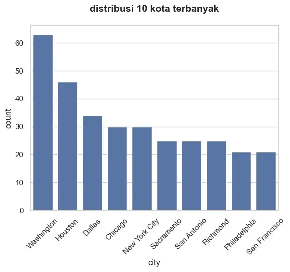
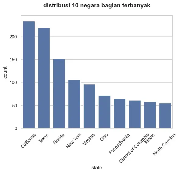
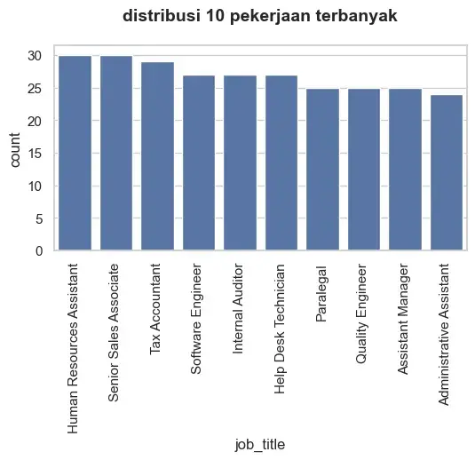
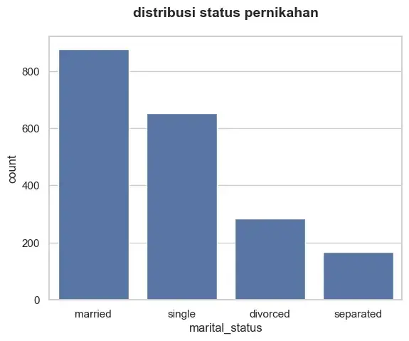
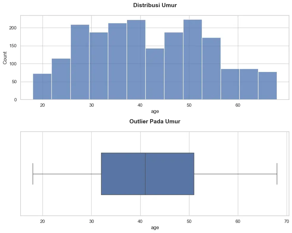
2. Bivariate Analysis
In this stage, I analyzed relationships between two variables to identify patterns and potential correlations. Analysis performed are Age vs Marital Status, and Age vs Job Title. Visualization to be created is boxplot.
#3. section ini berisi analisis bivariate
#age vs marital status
sns.boxplot(data=dataku, x="marital_status", y="age")
plt.title("distribusi umur berdasarkan status", fontsize=14, fontweight="bold", pad=20)
plt.tight_layout()

#age vs job title
sns.boxplot(data=dataku, x="job_title", y="age", order=dataku["job_title"].value_counts().head(5).index)
plt.title("distribusi umur berdasarkan 5 pekerjaan terbanyak", fontsize=14, fontweight="bold", pad=20)
plt.xticks(rotation=45)

plt.tight_layout()The following are the results image of the bivariate analysis.
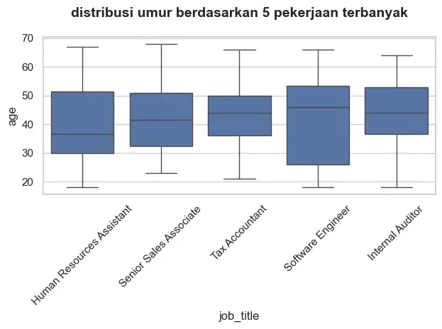
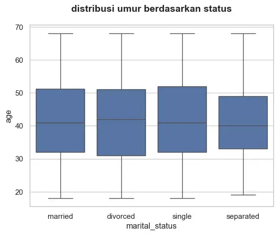
3. Time-Based Analysis
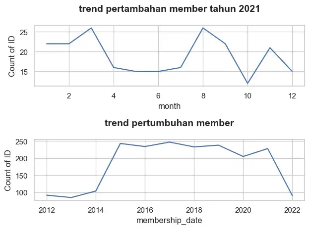
I analyzed membership trends over time using the membership_date column to observe member growth patterns. Analysis performed is Membership trend over time using Lineplot.
#4. section ini berisi analisis waktu
#membership_date
dataku["membership_date"] = pd.to_datetime(dataku["membership_date"])

plt.subplot(2,1,1)
data_2022 = dataku[dataku["membership_date"].dt.year == 2021].copy()
data_2022["month"] = data_2022["membership_date"].dt.month
sns.lineplot(data=data_2022, x="month", y="id", estimator=len)
plt.title("trend pertambahan member tahun 2021", fontsize=14, fontweight="bold", pad=20)
plt.ylabel("Count of ID")

plt.subplot(2,1,2)
sns.lineplot(data=dataku, x=dataku["membership_date"].dt.year, y="id", estimator=len)
plt.title("trend pertumbuhan member", fontsize=14, fontweight="bold", pad=20)
plt.ylabel("Count of ID")

plt.tight_layout()The following are the results image of the membership analysis.
Key Insights
I summarized the main findings discovered during the exploratory data analysis process.
- Age: The population is predominantly composed of individuals aged between 30 and 50 years old.
- Marital Status: Most individuals are either married or single.
- City: The top three cities with the highest number of individuals are Washington, Houston, and Dallas.
- State: The majority of individuals come from the states of California, Texas, Florida, and New York, each with more than 100 individuals.
- Job: The most common occupations are Human Resources Assistant (HRA), Senior Sales Associate, and Tax Accountant. Software Engineer is associated with the youngest individuals, with a minimum age of around 25 years old, while Tax Accountant has the highest minimum age, approximately 35 years old.
- Member Trend: The number of members showed a sharp year-over-year increase in 2015, growing by approximately 250% compared to 2014. The trend remained relatively stable until 2021, before experiencing a significant decline in 2022, dropping to fewer than 100 members.
Challenges & What I Learned
Challenges
- Deciding which missing values should be cleaned or retained based on business rules
- Choosing the most suitable visualization method for different data types
- Detecting unrealistic dates in the membership_date column
- Identifying inconsistent text formatting across several categorical columns
Limitations
- Outlier handling was limited to identification and basic correction
- The project focuses only on exploratory data analysis (EDA) and not predictive modeling
- The dataset size is relatively small compared to real-world production datasets
What I Learned
- Data cleaning is one of the most critical stages in data analysis
- Regular expressions (regex) are very useful for pattern-based cleaning
- Exploratory Data Analysis (EDA) helps uncover patterns before deeper analysis
- Understanding the dataset is just as important as creating visualizations
- Real-world datasets are often messy and require flexible cleaning approaches
Conclusion
The dataset was first processed through several data cleaning steps to improve data quality and consistency before analysis. This process included handling missing values, correcting inconsistent formats, removing duplicates, and preparing the dataset for visualization and exploratory analysis. These steps helped ensure that the analysis results were more accurate and reliable.
The analysis shows that the club member population is mainly dominated by individuals aged 30–50 years old, with most members being married or single. The highest number of members comes from California, Texas, Florida, and New York, while occupations such as Human Resources Assistant, Senior Sales Associate, and Tax Accountant appear most frequently in the dataset. In addition, membership growth increased sharply in 2015 before remaining relatively stable for several years, followed by a significant decline in 2022.
Changelog
V1.0 – First release (27 May 2026)
- Created a project and article


How Bad Was the Layoff Wave? Analyzing Global Layoff Trends Using PostgreSQL
Exploring Python Through a Simple Cafe POS System